Discrete Probability Distributions
Representing Probability Distributions
MINDS ON
 Consider the Following
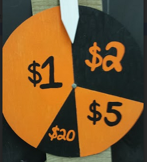
For the spinner, how much would you expect to win every time you spin it? Why do you think this might be?
ACTION
The question of expectations in games of chance require us to look at the outcomes and their probabilities. It is not as simple as saying "I expect to win" or "I expect to get lucky." We know from the Law of Large Numbers that all luck will even out and we will get precisely what we expect. So the question is "What do you expect?"
Expected Value is Average
The easy answer is that you should expect to get the average of all the outcomes. The average is calculated by adding up all of the outcomes and dividing by the total number of possible trials, just as it is when you are finding any average.
So for the spinner, what we expect to win won't be $1 or $2 or $5 or $20. It will be the average. However, could you calculate the average by saying:  Why would this not be correct the average? Are all outcomes equally likely?
We need a way of giving more weight to the $1 prize and less weight to the $20 prize.
 Revisit your Thinking
Brainstorm a way that you can find the average on the spinner so that each segment has different weights. Try and articulate it in your own words.
Revisit your Thinking
Did you think that you needed more information?
The angles in the circle are 145, 110, 70 and 35. Go back to your Portfolio and see if you can create the solution.
Discrete Probability Distributions
To formalize a way to calculate what you expect to happen, you need to organize probability scenarios, like the spinner, and display them to get a better understanding of what is happening. The spinner, in a way, is almost already organized graphically as a pie chart, so it gives you a way to see the probabilities. Some situations won't be that easy to see. As you saw in the first two units of this course, and by exploring games in the Games Fair Interactive tool, some probabilities can be difficult to calculate.
Definition: a probability distribution is a discrete function (definition:a relationship between two variables such that when you input a value, you get one and only one output.) that describes all of the possibilities of a probability scenario.
You will recall functions from Grade 11 as graphs, tables or formulas where you can find a y-value for each x-value you input.
Two definitions that we will come back to later in the course:
-
Discrete functions: when there are only a certain number of inputs. Discrete variables are obtained by counting, so there are only certain values that the inputs can take. For example: When rolling a die, the inputs could be the number rolled on the die, and the output would be the probability of the roll. A common misconception is that discrete functions can only involve whole numbers. However, shoe sizes fit the definition of a discrete variable as they only take certain values but could include half sizes. Example: size 7.5.
-
Continuous functions: when there are an infinite number of inputs. Continuous variables are obtained by measuring, so there is no limitation on the input value. For example: When looking at baby weights, the inputs could be the weight and the output could be the probability that a baby is that weight. Any decimal point could be entered for weight and only relies on the accuracy of the measuring tool. Continuous variables are a very interesting discussion in probability and will be the focus of the final unit of this course, after you develop some pre-requisite statistics knowledge.
The nice thing about discrete probability distributions is that there are only certain inputs and so they can be represented as a probability distribution table (table of values) or a bar graph and we can see all the possible values.
Uniform Distributions
The easiest type of probability to deal with is the probability where all outcomes are the same. This would be the case for the spinner, if all of the sections were equal. You will use this probability to lay some foundation for understanding distributions.
 Example
Consider the number when rolled on a single, 6-sided, die.
For each input: {1,2,3,4,5,6} we get the same output: 1/6. There are no other possible outcomes, and all the probabilities add to 100%.
This is a table of values and it represents the probability function which we call a "Discrete Probability Distribution."
|
Possible Outcomes: Number on die |
Probability |
|---|---|
|
1 |
1/6 |
|
2 |
1/6 |
|
3 |
1/6 |
|
4 |
1/6 |
|
5 |
1/6 |
|
6 |
1/6 |
You can also represent the distribution as a bar graph:
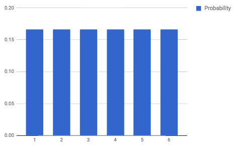
and probabilities are on the side.
Discrete Random Variables
In the previous units, you have called the set A the set of all successful outcomes and the set S as the set of all total outcomes. When discussing Probability Distributions, you will talk about the set X as the set of all possible outcomes. This helps redefine the total outcomes as the input variable, X, which we are used to seeing when talking about independent variables. (definition:The variable in a relationship that works as the input variable as it the output depends on it.)
For the die roll, the discrete random variable X (upper case) has specific values that are labelled x (lower case).
X = {1,2,3,4,5,6} and x can equal 1,2,3,4,5 or 6.
This allows you to speak in both general terms and specific terms by just changing the case of the "x."
Because the expected value is a general idea, the average of the entire function, we use the upper case "X."
So, it does seem confusing, but only initially, and should make more sense with some examples.
|
x |
P(x) |
|---|---|
|
1 |
1/6 |
|
2 |
1/6 |
|
3 |
1/6 |
|
4 |
1/6 |
|
5 |
1/6 |
|
6 |
1/6 |
The uniform distribution also has a formula, however, not all discrete distributions do. Here, P(X) = 1/6 because all probabilities are the same.
Expected Value Formula
Now, when calculating the average roll on a die, adding up the outcomes and dividing by the total makes sense.
Notice the E(X) is used with an upper case X because it is a general equation that represents the entire scenario. Also, notice that, although you can't roll a 3.5, that is the average, so that is what we expect. If you rolled the dice over and over, the Law of Large Numbers says, your average roll will be 3.5
You may have come up with the idea of taking the percentage of each outcome and adding them up. This is called the weighted average and it gives us a formula for the expected value:

 where
where is called "Sigma" and is the symbol for Sum, and where x starts at 1 and goes to n (the total number of trials).
A simpler way to show this is:
 where
where  means "add up xP(x) for each x value"
Back to the example of the die roll, a third column in the table best demonstrates this:
|
x |
P(x) |
xP(x) |
|---|---|---|
|
1 |
0.16667 |
0.16667 |
|
2 |
0.16667 |
0.33333 |
|
3 |
0.16667 |
0.50000 |
|
4 |
0.16667 |
0.66667 |
|
5 |
0.16667 |
0.83333 |
|
6 |
0.16667 |
1.00000 |
|
Total |
1.00000 |
3.50000 |
This method of creating the 3rd column gives you a process for finding the expected value. You just need to make sure that you still understand it as an average outcome over time. It also gives us a process for finding the expected value (average) when the probabilities are non-uniform.
Non-Uniform Probability Distributions
In this unit, you will start to see how the Games Fair games in the Interactive tool were created.
Record your work
Take a moment to play the Three Prize Roll in the Games Fair.
In this game, you win 10 points if you roll a 2, 20 points if you roll a 4 and 28 points if you roll a 6. The cost to play the game is 10 points. Would you play this game? What, on average, do you expect to win each time?
Create the probability distribution chart for the 4 outcomes (0, 10, 20, 28) and a bar graph. Calculate the expected value using the chart. Was your expected value hypothesis correct? Would you play this game?
GamesFair
Creating a Game
The exciting part about this unit is that you almost start to get to see how games of chance, like those people would see in a casino or scratch ticket, are created.
Definition: A fair game is a game where the expected value is equal to the cost of the game. If the cost of the game is already factored into the outcomes, the expected value is 0. When games are created, it is important that the game isn't paying out more than what was charged for the game. In essence, the creator of the game wants to make sure the game is NOT fair, but people are still enticed to play because of the hope of winning.
Example
Considering flipping 3 coins, or 1 coin 3 times. The number of possibilities can be found out from a tree diagram or using the slot method. There are 2 possibilities for each coin, so 8 in total. Now, if you don't keep track of the results on each individual coin and just count how many heads and tails you have, you could get the following: 3 Tails, 3 Heads, 2 Heads and 1 Tail, 2 Tails and 1 Head. It is more likely to get 2 and 1 because there are 3 ways to do it, versus only 1 way for you to flip all the same.
The following is a video discussing how to create the distribution table, but showing the power of a spreadsheet when creating a game. In this first table, X is a random variable and represents the number of heads you can get. In the second table, X becomes the number of points scored, which is based on the number of heads.