Continuous Probability Distribution: The Normal Distribution
Continuous vs. Discrete
MINDS ON
 Share Your Thoughts
When a company fills an aluminum can with pop for sale, they print the mL on the can. Often, a can is set to fill up 355 mL of liquid.

What is the probability that a pop can, which has been filled with 355 mL of liquid, and advertises 355 mL, actually contains exactly 355 mL?
ACTION
Recall the following information from Unit 5.
Continuous vs. Discrete
The difference between the two is whether or not they are obtained by measuring or counting.
Continuous Data
Definition: Continuous data is data that is obtained by measuring. You can measure data in different ways, including time and distance. Because there is always a data point that can exist between two data points and there is a possibility of infinite data points, measured data is continuous and organized into intervals.
 Example
How long does it take you to get to school?
Your answer here could be 20 minutes for example. Say the intervals the data was being organized into were:
- 15-20 minutes,
- 20-25 minutes,
- 25-30 minutes.
What interval would your time go into? You would have to look at the accuracy of your time.
As a continuous data point, 20 minutes is either higher than 20 (20.000000001 for example) or lower than 20 (19.999999999 for example). So you would always be able to decide which interval you belong to.
Discrete Data
Definition: Discrete data is data that is obtained by counting. This type of data was what you focused on in the first half of this course. Discrete data points, unlike continuous ones, do not have points between points. There are a finite number of possibilities.
Examples
- How many heads do you get when you flip a coin 3 times? The only possibilities are 0,1,2 and 3. There are no values between these.
- What percent did you score on your G1 driver's test? Here, even though the numbers can be decimals, they were obtained by counting the score. Making the score a percent does not change it from a discrete data point to a continuous one. Even if the instructor used half or quarter points, it is not possible to score every value on the number line (even decimals) between 0 and 40.
Calculating Probabilities
We have spent the first half of the course learning about how to calculate probabilities for discrete distributions, by counting the total number of possible ways to arrive at a specific outcome and divide by the total possible ways to arrive at all outcomes. As discrete variables are measured by counting, discrete probabilities are calculated by counting.
In a discrete probability histogram, each of the outcomes would have its own unique probability, and you can read the probabilities of each outcome off of the graph.
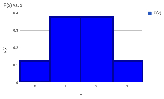
number of heads flipped when flipping 3 coins.
The focus of this unit will be on calculating probabilities for continuous variables. The probabilities for continuous variables are calculated by summarizing data that shows up on an interval.
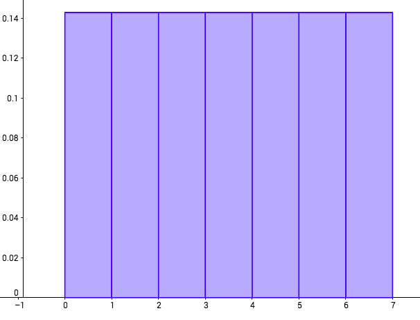
Definition: Similar to a discrete probability histogram, a continuous probability density graph shows us the percentage or probability of different amounts occurring except the histogram is shown on intervals. We can find the probabilities of specific intervals by finding the area of the graph between those intervals. What makes the probability density graph very useful is the fact that the area of the bars add to 1.
This is most easily seen in a graph of uniformly distributed data:
 Record Your Work

Answer the following questions about the uniformly distributed graph:
- What is the probability that a wait time will be between between 2 and 5 minutes?
- What is the probability that a wait time is more than 6 minutes?
- What is the probability that a wait time is less than 2.5 minutes?
- What is the probability that a wait time is exactly 4 minutes?
Compare your answers to the solutions below. What did you get correct? What are you having trouble with?
Solutions
- 30%
- 60%
- 25%
- 0%
Now, often, you will see a probability density graph with intervals that are not a width of 1. See the following graphing on the distribution of teacher ages at an Ontario High School.
The height of each bar is 0.1428.
Age is a continuous variable, and for this example, teacher's ages would be the time since they were born. In other words, if a teacher was 35, they would be in the 35-40 interval. If a teacher was 40, they would be in the 40-45 interval.
Now, the area would not work here to give the probability of intervals other than the ones given. The total area under the curve is  or 5 times what it should be.
This is because the interval size is 5. What we can do is take each of the interval boundaries and call 25 = 0, 30 = 1, 35 = 2 and so on....
This would be the same as calling 5 years equal to 1 unit.
This would be illustrated in the following graph, by taking each age, subtracting 25 and then dividing by 5:
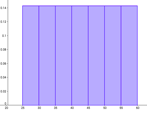
The height of each bar is 0.1428.
The units represent every 5 years, starting at age 25.
Now we can calculate probabilities involving the teachers by using the area of the bars because the total area is: 
You will calculate probabilities for this graph in the quiz in this activity.

A common question for discrete probabilities is whether or not the question includes the number given. For example, if you wanted to find the probability of less than 2 heads flipped on 3 coins, you would have to ask whether or not 2 heads is included. Asking "What is the probability of 2 or less heads on the flip of 3 coins?" is different from asking "What is the probability of less than 2 heads on the flip of 3 coins?" For the first, we could write:  . For the second we could write
  which is the same as
  .
.
For continuous probabilities, since the probability of any specific value is 0%, the probability that a number is less than a certain number is the same as the probability that a number is less than or equal to that certain number. In other words,  is the same as
  . The area of the bars over these intervals are the same.
Challenges with Continuous Variables
Unlike discrete variables like the ones we saw in the first half of this course, continuous variables do not have theoretical probabilities associated with them. Often we can only base our probabilities on past data and create a histogram based on a sample of the data. The length of time it takes you to get to school, for example, can be modelled after collecting a sample of the times it takes you to get to school. There will be some variability(definition:The extent to which numbers are different.) in the data, requiring a measure of the mean and the standard deviation, which we will see in the remainder of the unit. There is also a need to assume that the data will behave in a certain way, by being normally distributed around the mean.
In Activity 4, you will see some data for Hurricane wind speeds. Now, since it is impossible to calculate the theoretical probability of a Hurricane having a wind speed of greater than a certain amount, the best we can do is to make a mathematical model based on the past data that we have. This may include only a sample of the data, which will need to represent the population. It may also require us to use data that may not be as accurate, because it was calculated by different sources.
CONSOLIDATION
 Application and Thinking
Revisit the 100m results discussed in the Introduction. Based on what you have learned in this activity, did Jeneba Tarmoh and Allyson Felix actually tie for 3rd?
What would you recommend to avoid this in the future?