The so-called "Law of Frequency of Error" that Sir Francis Galton mentions in the quote from the introduction is the idea that we can predict, with a high number of data, the amount that natural things, which are seemingly chaotic, that deviate from the average.

The Normal Curve

In naturally occurring variables, we can assume that the modal interval will lie in the middle of the data, at the average.  Then points will fall above and below the average with decreasing frequency as they get farther from the average.  The "Law of the Frequency of Error" tells us that for every really high point from the average, there will be a very low point, making a symmetric curve on both sides.

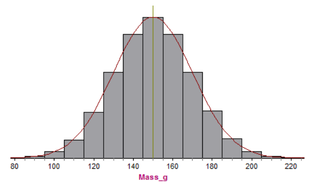
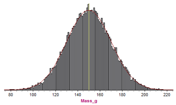
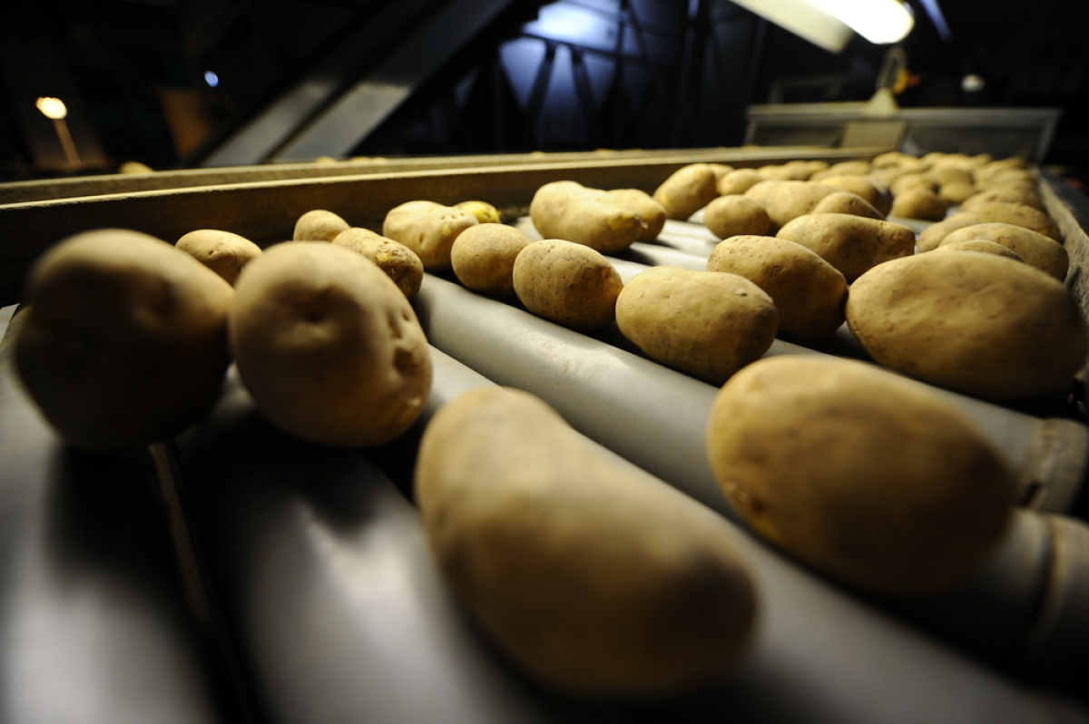
In the following example, the mass of 21000 potatoes, in grams is recorded with an average mass of 150 g and a standard deviation (definition:The distance a typical point is from the average.) of 20 g.  The standard deviation shows how far points ended up above and below the average.

For 21000 potatoes, an interval size of 10 g is used, giving the following histogram.  The Normal Curve has been placed over the probability density histogram so you can see how well it describes the data.

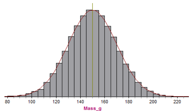
If you decrease the interval size to 5 g, you can see, similar to the last activity, the improved fit of the normal curve:

Decreasing to 2 g, it becomes harder to see gaps between the curve and the histogram:

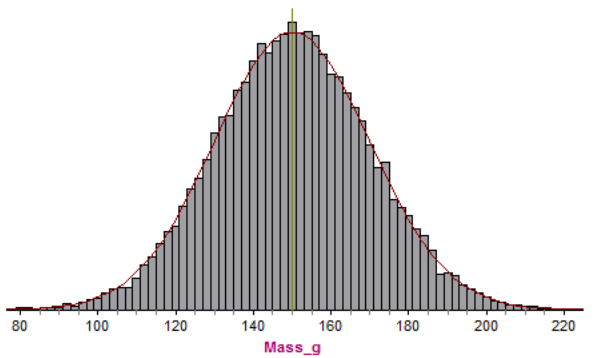
When the interval size is 1 g, the curve almost exactly covers the histogram:

Rule of 68, 95, 99.7

When many data points are taken and the mean and standard deviation are calculated, we can predict that the data and the probability density graph will follow a predictable curve, and we no longer need the rectangles, and their areas to calculate probabilities.

The curve is always the same curve, no matter the context, as long as the data can be expected to be normally distributed.  What customizes the curve is the standard deviation and mean.

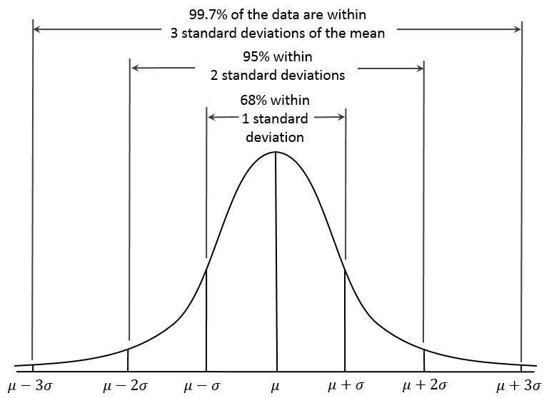
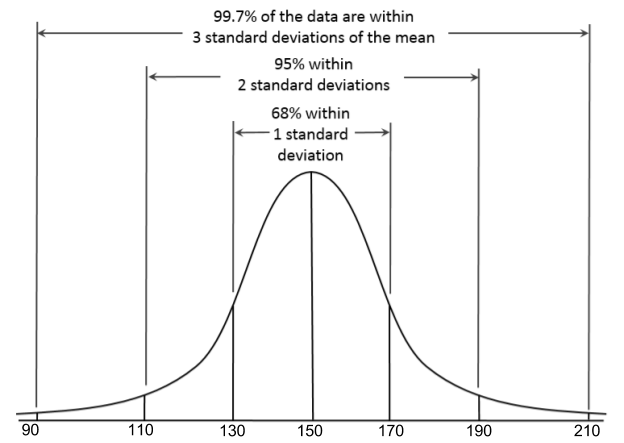
For every normal curve, we can say that approximately 68% of the data lies within 1 standard deviation from the mean.  In this example, 68% of the potatoes are between 130 and 170 g. 

Now, if we called  the random variable that represent the mass of potatoes, we would say that  is approximately normally distributed with a mean of 150 and a standard deviation of 20.  We say that in symbols by writing: 

We can also write:  

We also know that 95% of the data is within 2 standard deviation from the mean.  In this example, 95% of the potatoes are between 110 and 190 or 

Finally, we know that 99.7% of the data is within 3 standard deviations from the mean.  In this example, 99.7% of the potatoes are between 90 and 210 g or 

This rule of 68, 95, 99.7 is shown in the following image.  Recall that  represent the population mean and  represents the population standard deviation.  In general, we can show that a random variable, X, is normally distributed with a mean, , and standard deviation, , by writing  where  represents the variance.

The benefit of knowing the rule of 68, 95, and 99.7 is that you can calculate many other probabilities just from those three numbers.

Work through the following interactive to help understand how to uncover many other probabilities:

NormCurve

Long Description