Acceleration

Acceleration is the rate at which an object’s velocity changes. It is given the symbol ( $\vec{a}$ ), and is measured in metres per second per second, or metres per second squared (m/ $s^{2}$ ). In other words, it is how the velocity (measured in m/s) changes per second.

Note that because acceleration is based on change in velocity, which is a vector quantity, acceleration is a vector quantity as well. Direction must always be included when discussing acceleration.

Uniform motion is motion in which the velocity does not change. Non-uniform motion occurs when the velocity of an object is not constant: the object speeds up or slows down during its motion, or changes direction. The motion we’ll be looking at in this activity will all be non-uniform, however, we will only be looking at examples where the magnitude of the velocity changes -- we will keep everything in one dimension.

Uniform Motion vs. Non-Uniform Motion

How can we tell these two types of motion apart?

Here is the data of an object that is undergoing uniform motion.

Time (t) in s	Position ( $\vec{d}$ ) in m [S]
0	0
10	20
20	40
30	60
40	80
50	100
60	120
70	140

The amount of distance covered is the same for each 20 second interval. If we were to graph this, the slope of each line segment would be the same:

$\vec{v}= \frac{\Delta \vec{d}}{\Delta t}$

$\vec{v}= \frac{100m[S]-80m[S]}{50s-40s}$

$\vec{v}= \frac{20m[S]}{10s}$

$\vec{v}= 2m/s[S]$

And the graph would look like this:

This is a position-time graph for an object undergoing uniform motion.

What does the position-time graph look like for an object that’s accelerating? Let’s create a scenario with non-uniform motion.

Position-Time Graph - Acceleration

We’ll start with the same time data as above, but this time, you will create the position data. In the original set of data, the object increased its distance by 20 metres every 10 seconds. In this case, the object will need to cover greater and greater amounts of distance in each 10-second interval.

Time (t) in s	Position ( $\vec{d}$ ) in m [S]
0	0
10
20
30
40
50
60
70

Now, graph your data. Compare what you see in your graph with the graph of uniform motion earlier in this activity.

Create a reflection, and record your answers to the following questions:

How does the shape of your non-uniform motion graph differ from the uniform motion graph?
What do you think the position-time graph of an object that was slowing down might look like?

Submit Your Work

Take a look at the following position-time graph -- it might resemble the one you created.

This is a position-time graph of an object undergoing acceleration

Can you see a difference between the rate of change (slope) in the first segment and the rate of change (slope) in the last segment? In each segment, actually, the rate of change is getting a little larger each time, and the slope is getting a little steeper.

And, if rate of change of a position-time graph is the object’s velocity, that means that the object is going a little faster in each segment.

An object that is slowing down might have a graph that looks like this:

This is a position-time graph of an object negatively accelerating, or slowing down.

In the above case, the greatest rate of change (greatest velocity) is the first segment, and then the slope decreases (the velocity decreases) throughout the rest of the object’s motion.

In general, a curved position-time graph indicates non-uniform motion.

When the velocity is constant, you are aware of what a position-time graph looks like -- a straight line, slanted up. When it comes to non-uniform motion, if we want a visual representation of how that velocity is changing, we may want to change what we graph.

Instead of a position-time graph, we can create a velocity-time graph. In both cases, time is our independent variable, and is on the horizontal axis. With a velocity-time graph, though, the instantaneous velocity is on the vertical axis. Let’s take a look at what this looks like.

For our original object moving in uniform motion, this is what the velocity-time graph would be:

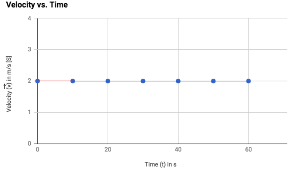
This is a velocity-time graph of an object undergoing uniform motion

This graph may seem strange, as it represents a horizontal line at the value of 2 m/s [S]. But remember that the object is moving in a uniform way, at 2 m/s the whole time, in the same direction. If there is no change in velocity (i.e., the velocity is constant), then it makes sense that the object’s velocity-time graph always indicates a velocity of 2 m/s [S].

An object that isn’t moving in uniform motion will have different velocities indicated on its velocity-time graph. Here is a graph that matches the motion of our unknown object moving with non-uniform motion.

This is a velocity-time graph of an object accelerating at a uniform rate

By reading points off the graph, we can see that the object is accelerating: at 20 seconds, the object is moving at 2 m/s [S], but then at 40 seconds, the object is moving faster, at 4 m/s [S]. At 60 seconds, the object is travelling at 6 m/s [S].

Can we find the rate of this acceleration? Of course! Any time we have a linear graph, we can find the rate of change, just like we did in Activity 2.

Let’s find the rate of change between the points (20, 2) and (40, 4).

$Rate of Change= \frac{\Delta y}{\Delta x}$

$Rate of Change= \frac{y_{2}-y_{1}}{x_{2}-x_{1}}$

$Rate of Change= \frac{4m/s[S]-2m/s[S]}{40s-20s}$

$Rate of Change= \frac{2m/s[S]}{20s}$

Rate of Change= 0.1m/s/s[S]

For every second that passes, the object is going 0.1 m/s[S] faster than it was the second before. We could also write this answer as 0.1 m/ $s^{2}$ [S].

Did You Know?

Even though it’s commonly used in everyday life, physicists rarely use the term “deceleration.” Instead, they say that an object that is slowing down undergoes “negative acceleration.” Can you guess why?

Let’s repeat our rate of change calculation for an object that is slowing down. Here’s the position-time graph we saw earlier for an object getting slower and slower…

This is a position-time graph of an object with negative acceleration

If we take the slope of each segment, and plot those values in a velocity-time graph, we get the following:

This is a velocity-time graph of an object undergoing negative acceleration at a uniform rate.

Question

Using the graph above, choose two points, and determine the rate of change, then check your answer.

Let’s use the points (0, 30) and (40, 10):

$Rate of Change= \frac{\Delta y}{\Delta x}$

$Rate of Change= \frac{y_{2}-y_{1}}{x_{2}-x_{1}}$

$Rate of Change= \frac{10m/s[S]-30m/s[S]}{40s-0s}$

$Rate of Change= \frac{-20m/s[S]}{40s}$

Because the object is slowing down, when we calculate the rate at which its velocity is changing, we see it is experiencing a negative acceleration. Every second, the object is moving at a speed 0.5 m/s [S] slower than it was the previous second.

Negative acceleration indicates an object is slowing down.

Reflection

Think back to the Minds On task at the beginning of this activity -- you were asked to guess when the parachutist would experience the greatest acceleration.

Go back to your initial reflection on the parachutist and remind yourself of what you guessed. After what we’ve learned about acceleration, would you like to change your mind? If so, indicate this in your reflection with your reasoning for having a different answer now.

Were you right? Watch the video below to see!

After watching the video, add to your reflection by recording the answers to the following questions:

Did you correctly guess the greatest acceleration? If not, what did you not take into consideration when making your guess?
In the video, they look at an acceleration-time graph. In our examples in this activity, our objects were all undergoing uniform acceleration (accelerating at the same rate the entire time). What do you think the acceleration-time graph would look like for our objects?

Go To Portfolio

Practice

If acceleration is the rate of change of an object’s velocity, we can derive a formula for acceleration from a velocity-time graph:

$\vec{a}= \frac{\Delta y}{\Delta x}$

Because velocity ( $\vec{v}$ ) was on the y-axis, and time (t) was on the x-axis, we can write:

$\vec{a}= \frac{\Delta \vec{v}}{\Delta t}$

$\vec{a}= \frac{\vec{v_{f}}-\vec{v_{i}}}{t_{f}-t_{i}}$

Let’s try to solve an acceleration problem. Don’t forget to use the GRASP method!

A car accelerates from a velocity of 17 m/s [W] to a speed of 25 m/s [W] in 22 seconds. What is the car’s acceleration?

Answer

Given:

We are given the following measurements:

$\vec{v_{i}}= 17m/s[W]$
$\vec{v_{f}}= 25m/s[W]$
$\Delta t= 22s$

We chose $\Delta t$ because the question gives us the total time during which the change in speed occurs. We could have also used ( $t_{f}-t_{i}$ ), with the values of $t_{f}= 22s$ and $t_{i}=0s$ , assuming the time started when the car started changing its velocity from 17 m/s [W] to 22 m/s [W].

Required:

We are asked to determine the acceleration:
$\vec{a}= ?$

Analysis:

We know that acceleration is the change in velocity over time. In other words, it is the change in velocity divided by the change in time.

Solution:
$\vec{a}= \frac{\vec{v_{f}}-\vec{v_{i}}}{\Delta t}$

$\vec{a}= \frac{25m/s[W]-17m/s[W]}{22s}$

$\vec{a}= \frac{8m/s[W]}{22s}$

$\vec{a}= 0.36m/s/s[W]$

Paraphrase:

The car accelerated at 0.36 metres per second per second westward. We could also say that the car’s speed increased by 0.36 m/s [W] every second.

Try another one. This time, we will have to rearrange the formula in order to get what we need.

A ball starts rolling down a ramp at 2.1 m/s [down], and accelerates at 1.5 m/ $s^{2}$ [down]. It gets to the bottom of the ramp 3.5 seconds later. What was its velocity at the bottom of the ramp?

Answer

Given:

We are given the following measurements:
$\vec{v_{i}}= 2.1m/s$

$\Delta t= 3.5s$

$\vec{a}= 1.5m/s^{2}$

Required:

We are asked to determine the final velocity:

$\vec{v_{f}}= ?$

Analysis:

We know that acceleration is the change in velocity over time. In other words, it is the change in velocity divided by the change in time. If we are given the acceleration, the initial velocity, and the time, we can determine the final velocity.

Solution:

$\vec{a}= \frac{\vec{v_{f}}-\vec{v_{i}}}{\Delta t}$

We have all the variables necessary for this calculation already, but will need to rearrange the formula in order to solve for final velocity.

Multiplying both sides by $\Delta t$ :

$\vec{a}\Delta t= \vec{v_{f}}-\vec{v_{i}}$

Adding ( $\vec{v_{i}}$ ) to both sides:

$\vec{a}\Delta t+\vec{v_{i}}= \vec{v_{f}}$

We can now solve for final velocity:

$\vec{v}_{f}= \vec{a}\Delta t+\vec{v}_{i}$

$\vec{v}_{f}= (1.5m/s^{2}[down])(3.5s)+2.1m/s[down]$

$\vec{v}_{f}= 5.25m/s[down]+2.1m/s[down]$

*Note that when we multiply acceleration and time, the resulting units are m/s, which allows us to add the 5.25 m/s [down] and the 2.1 m/s [down] since they have the same units and direction.

$\vec{v}_{f}= 7.4m/s[down]$

Paraphrase:

The ball’s velocity at the end of the ramp was 7.35 m/s [down].

Questions

Try the following questions to see if you’ve got it!

Alouette I was Canada’s first satellite. Launched in 1962, it made Canada the third nation in the world to launch a satellite into space. It was launched with the help of NASA on a two-stage Thor-Agena rocket. Answer the following questions related to this space milestone.

A rocket blasts off from the surface of Earth at an acceleration of 21 m/s/s [up]. If its motion is graphed on a speed-time graph, the line it would produce would be
1. a flat horizontal line.
2. a straight line with a positive slope.
3. a straight line with a negative slope.
4. a bent line curving up.
Answer

Answer: b. a straight line with a positive slope.

The speed of the rocket is increasing at 21 m/s/s [up]. This means it increases by 21 m/s [up] each second (eg: 0 m/s [up], 21 m/s [up], 42 m/s [up], 63 m/s [up], ...). Thus, on a velocity-time graph, the points would be equally spaced going up, causing a constant positive slope.
Its initial acceleration was not actually 21 m/s/s [up]. If it went from rest to 660m/s [up] in a time of 12 seconds, its acceleration would be:
1. 42 m/s/s [up]
2. 27.5 m/s/s [up]
3. 110 m/s/s [up]
4. 55 m/s/s [up]
Answer

Answer: d. 55 m/s/s [up]
$\vec{a}= \frac{\vec{v}_{f}-\vec{v}_{i}}{\Delta t}$

$\vec{a}= \frac{(600m/s[up] - 0m/s[up])}{12s}$

$\vec{a}= \frac{660m/s[up]}{12s}$

$\vec{a}= 55m/s/s[up]$
Once the first stage burns out, it separates and fall back to Earth. Before the second stage starts burning, the rocket slows down for a short time. If the rocket slows from 1200 m/s [up] to 1140 m/s [up] over a period of 5.0 seconds, what is the acceleration of the rocket for this time between stages?
1. 36 m/s/s [up]
2. 12 m/s/s [up]
3. -12 m/s/s [up]
4. -36 m/s/s [up]
Answer

Answer: c. -12 m/s/s [up]
$\vec{a}= \frac{\vec{v}_{f}-\vec{v}_{i}}{\Delta t}$

$\vec{a}= \frac{(1140m/s[up]-1200m/s[up])}{5.0s}$

$\vec{a}= \frac{-60m/s[up]}{5.0s}$

$\vec{a}= -12m/s/s[up]$

The first stage separates from the rocket and begins to fall back to Earth. As it leaves, the rocket is travelling at 1200 m/s [up]. If it is slowing down at an acceleration of -5.5 m/s/s [up], how long will it take to slow down to a velocity of 0 m/s?
1. 60 s
2. 110 s
3. 220 s
4. 440 s
Answer

Answer: c. 220 s

$\vec{a}= \frac{\vec{v}_{f}-\vec{v}_{i}}{\Delta t}$

$\vec{a}\Delta t= \vec{v}_{f}-\vec{v}_{i}$

$\Delta t= \frac{(\vec{v}_{f}-\vec{v}_{i})}{\vec{a}}$

$\Delta t= \frac{(0m/s[up]-1200m/s[up])}{-5.5m/s/s[up]}$

$\Delta t= \frac{-1200m/s[up])}{-5.5m/s/s[up]}$

$\Delta t= -220s$

CONSOLIDATION

Summary:

Acceleration ( $\vec{a}$ ) is the rate at which an object’s velocity changes.
$\vec{a}=\frac{\Delta \vec{v}}{\Delta t}$
It is measured in metres per second per second (m/s/s or m/ $s^{2}$ ), and is a vector quantity.

A velocity-time graph illustrates how an object’s velocity changes over time. Time is the independent variable (on the x-axis) and velocity is the dependent variable (on the y-axis).

Non-uniform motion occurs when an object’s velocity (either the magnitude, or the direction, or both) is variable (i.e. the object undergoes acceleration).

Negative acceleration indicates an object is slowing down.

When analysing graphs:

A curved position-time graph indicates non-uniform motion.
A velocity-time graph with a positive slope indicates an object is accelerating.
A velocity-time graph with a negative slope indicates an object is negatively accelerating.
A velocity-time graph with a flat line (slope of zero) indicates uniform motion.

Motion (Kinematics)
Non-Uniform Motion, Acceleration, and Velocity-Time Graphs

MINDS ON

Reflection

ACTION

Acceleration

Uniform Motion vs. Non-Uniform Motion

Position-Time Graph - Acceleration

Did You Know?

Question

Reflection

Practice

Questions

CONSOLIDATION

Summary:

Motion (Kinematics)Non-Uniform Motion, Acceleration, and Velocity-Time Graphs

MINDS ON

Reflection

ACTION

Acceleration

Uniform Motion vs. Non-Uniform Motion

Position-Time Graph - Acceleration

Did You Know?

Question

Reflection

Practice

Questions

CONSOLIDATION

Summary:

Motion (Kinematics)
Non-Uniform Motion, Acceleration, and Velocity-Time Graphs